From Curves to Constraints: How Groth16 Proves a Computation Without Revealing Its Secrets
You have computed something that matters. A payment is authorized, a reserve is met, a batch of checks passed. You want someone else to accept the result without taking the private inputs. Groth16 is one way to do that. The proof is three group elements. The verifier checks one pairing equation.
This page follows one statement the whole way, the same one the companion episode uses. In a field of 101 elements, the prover knows a private x such that
The running numbers are x = 3 and public y = 35. Then x^2 = 9 and x^3 = 27. Every matrix, polynomial, and pairing check below is this same assignment, written in a new language.
The episode is written to work with your eyes closed. The lab is optional. It lets you change a number and see which layer breaks. The Groth16 module is a scalar-exponent shadow of the verification equation, not a cryptographic implementation. The setup trapdoors and the exponents are visible by design. It shows the algebra. It does not hide a witness, and it is not a proof you can trust.

Where the lab meets the audio
The five modules do not follow narration timestamps. They follow chapters. Pause, run the default example, then break one input on purpose.
- Curve group, chapter 2. Finite-field points, a modular slope, reflection, and the identity. Open it.
- Arithmetic circuit, chapter 4. Private x, public y, and the wires in between. Open it.
- R1CS, chapter 5. Three rows, one shared witness vector. Open it.
- QAP divisibility, chapters 6 and 7. Constraints, roots, and a zero remainder. Open it.
- Groth16 check, chapters 8 and 9. Setup factors, randomizers, proof elements, and the verifier’s own V. Open it.
Open the full lab. Each module keeps its own inputs. Changing x in the circuit does not change x in the R1CS. Next and Back step the animation. When focus is not in a form or a button, the left and right arrow keys do the same.
The re-paced episode is 59:19. Chapter starts: 00:00 intro, 03:33 the arithmetic universe, 05:22 elliptic curves as groups, 09:36 pairings, 13:24 compiling a computation, 17:53 R1CS, 21:43 from rows to polynomials, 29:49 recap, 30:46 why one secret point is tempting, 33:05 the structured reference string, 37:51 constructing the proof, 47:57 recap, 48:54 where zero knowledge comes from, 52:29 the developer’s workflow, 56:18 putting the layers in place.
The arithmetic is modular
Before the curve, fix the number system the circuit actually uses. \mathbb{F}_{101} is the integers modulo 101. Addition and multiplication wrap. 100 + 5 = 4 in this field, not 105. Every coefficient in the rank-one constraints and in the polynomials lives here.
That wrap is the whole warning. A field equation does not say “this is an ordinary integer in range” unless the circuit adds constraints that force the range. This example does not. The lab will happily compute a large x and show the wrapped result.
The same curve, two pictures
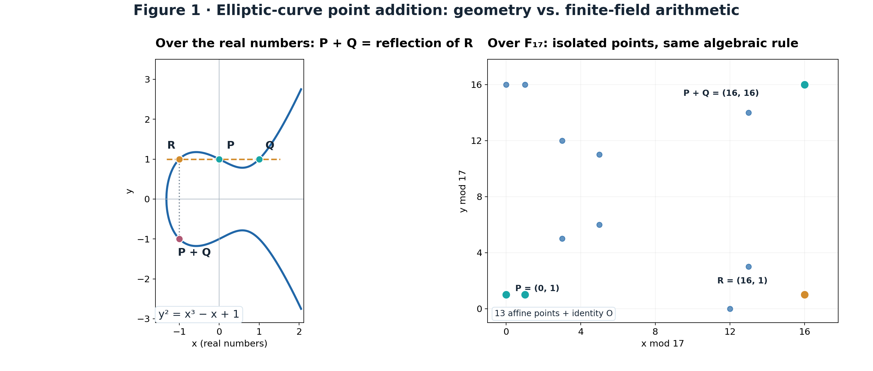
The curve in the figure is
Over the reals you can draw it. Take P = (0, 1) and Q = (1, 1). The chord through them meets the curve again at R = (-1, 1). The sum is the reflection of that third point across the x-axis: P + Q = (-1, -1).
Over \mathbb{F}_{17} the equation is the same and the drawing is not. Only the coordinate pairs that satisfy it are points. There is no continuous chord on the screen. The group law is the slope arithmetic. The same inputs give P + Q = (16, 16). Negation sends (x, y) to (x, -y). Adding a point to its inverse produces the point at infinity, the identity element O. There is no ordinary coordinate pair for that identity.
The highlighted third intersection in the lab is the algebraic result of the group law. It is not a claim that a Euclidean line on the page passes through the finite-field points.
Multiplication of a group element by an integer is repeated addition. A Groth16 proof element is a point in a curve group, an encoding of a scalar, not the scalar written in the clear. This toy curve is not a pairing-friendly parameter set. It is here so the group operation is visible.
Try it. In the module below, leave P = (0,1) and Q = (1,1) and step to the sum (16, 16). Then press Use P = Q and watch the tangent slope replace the chord slope. Then press Use Q = −P. The result is the point at infinity.
The addition formulas survive after the smooth picture is gone because they were field arithmetic the whole time. The drawing over the reals was one picture of that arithmetic.
What a pairing is for
A cryptographic curve has a coordinate field and a chosen prime-order subgroup whose scalars form another field. Circuit arithmetic for Groth16 runs in the scalar field. The proof elements are points. A pairing is a map
with
The verifier multiplies two hidden scalars by pairing the points that encode them, and does not learn a or b. That is the only reason the curve showed up. You do not need to construct a pairing to follow the rest of this page. You need the property: the check can multiply exponents that stay inside the group elements.
The same family of tools shows up when a vector commitment opens one position of a wide node. The Merkle and Verkle essay stops at the opening. This page is the pairing check those openings rely on.
Compile the expression into wires
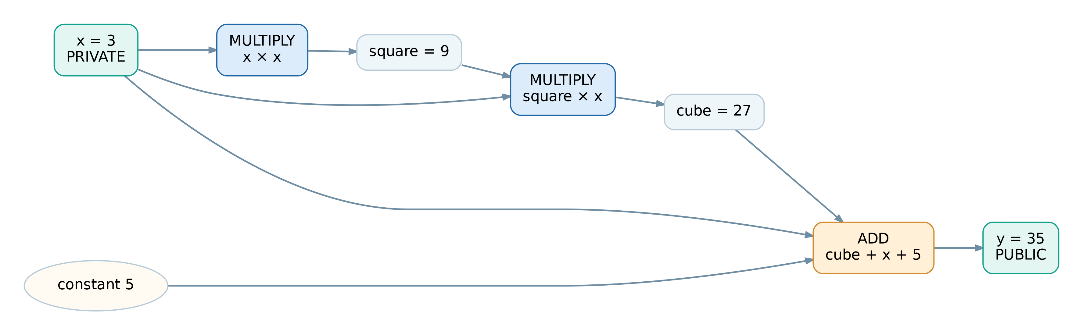
A prover does not hand the verifier source code and hope it gets run. The computation has to be a list of algebraic conditions. The statement is
The prover knows x. The verifier chooses y. The circuit names the intermediate wires:
With x = 3, the wires are s = 9, c = 27, and the computed output is 35. If the verifier’s y is 35, the claim holds. If the verifier sets y to 36, the gates still produce 35, and the claim is false. Zero knowledge does not enforce a condition you forgot to write down. The relation is the constraints.
Try it. Leave x = 3 and y = 35 and step through the gates. Press Set y = output + 1. The computed output does not move. The claim does. Set y to computed output puts the statement back. Try a larger x and watch the wires wrap modulo 101.
One witness, three rows
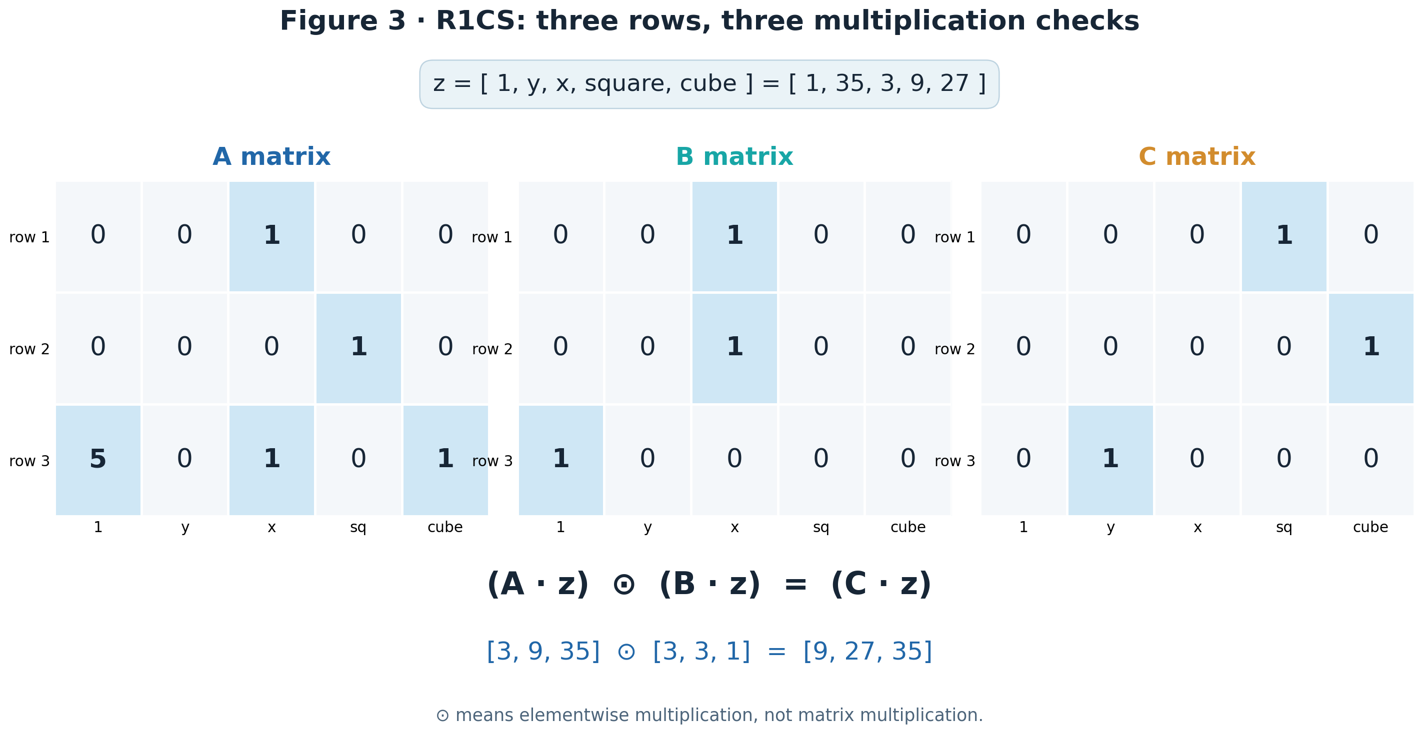
Rank-one constraint systems write each multiplication in the same shape. Row i demands
for one shared vector. Column order is constant term, public output, private input, square, cube:
The matrices are fixed by the circuit. Only z changes when the proposed computation changes.
        columns:  1  y  x  s  c

A     row 1       0  0  1  0  0
      row 2       0  0  0  1  0
      row 3       5  0  1  0  1

B     row 1       0  0  1  0  0
      row 2       0  0  1  0  0
      row 3       1  0  0  0  0

C     row 1       0  0  0  1  0
      row 2       0  0  0  0  1
      row 3       0  1  0  0  0
Dot those rows with the default z and the linear forms are
The elementwise product of Az and Bz is Cz. All three residuals are zero. Row 3 is the public check: (c + x + 5) \cdot 1 = y, which is (27 + 3 + 5) \cdot 1 = 35.
The numbers in z are a proposal. Nothing stops you from typing a square that is not x^2. Row 1 fails, and row 2 may fail with it. Public y is unchanged. A valid witness is an assignment to every wire that passes every row, not a claim about x alone. If the circuit never constrains s = x^2, the proof system will not invent that constraint. It will prove a different relation.
Try it. The module starts at z = [1, 35, 3, 9, 27]. Step the three rows, then press Corrupt square. Repair puts the wires back by recomputing them from x. Change only the cube and see which rows light up.
Roots, then a quotient
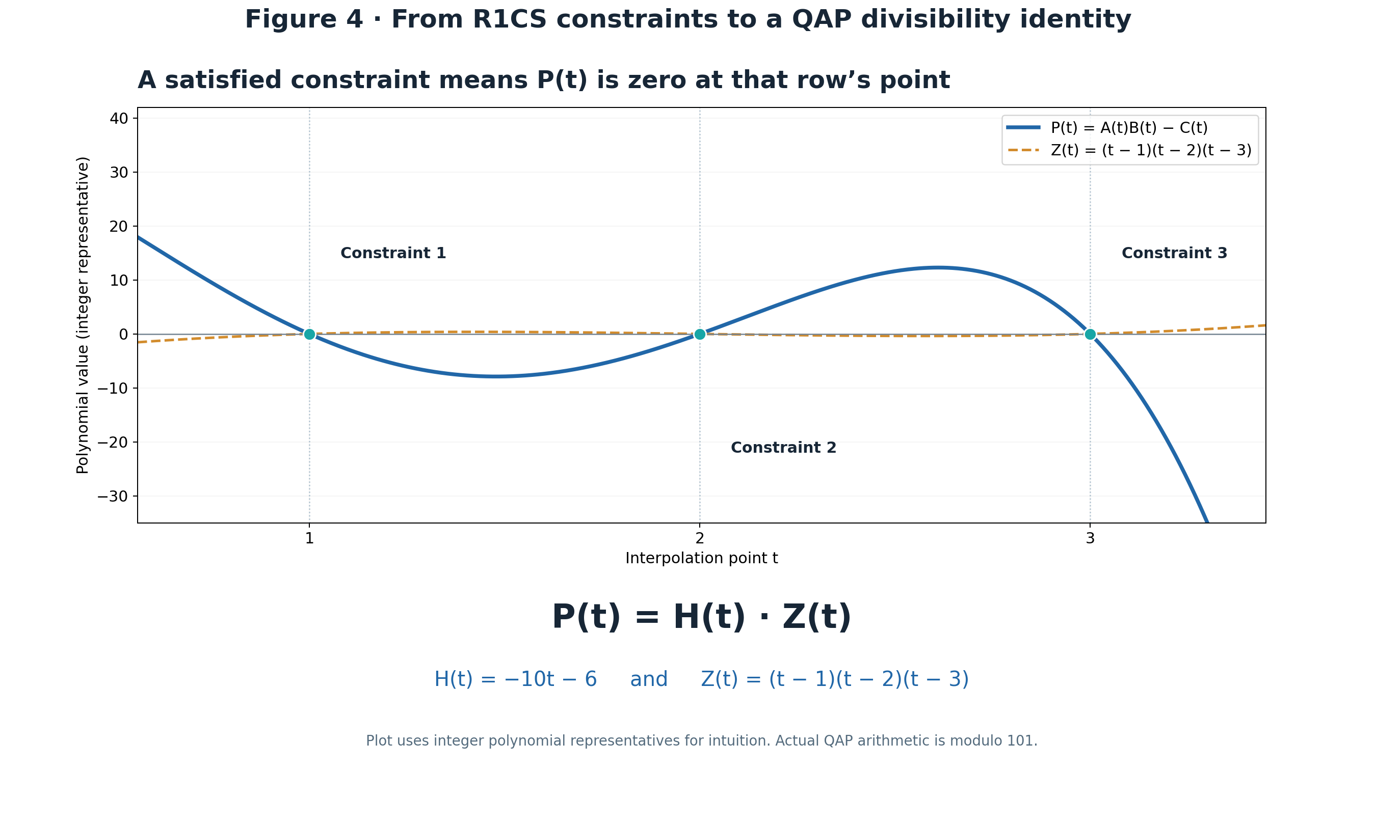
This is the bridge. The three rows become three test points in the same field:
Interpolation builds three witness-dependent polynomials A_z(t), B_z(t), and C_z(t) whose values at those points are the row calculations. For the default witness, one choice of representatives is
Read every coefficient modulo 101. Define the error polynomial and the vanishing polynomial:
Row i holds exactly when P_z(r_i) = 0. The points are distinct, so the factor theorem says these are the same claim:
Nothing new was assumed. The claim changed shape, not meaning. For this witness the quotient is H(t) = -10t - 6, which is 91t + 95 modulo 101, and the remainder is the zero polynomial. The identity A_z B_z - C_z = H Z holds over the integers for these particular representatives, so it holds in the field too. The exact coefficients matter less than the zero remainder.
At a point that is not a root, the same identity is a sanity check. P(4) = -276 \equiv 27 \pmod{101}, and H(4)\,Z(4) = (-46)\cdot 6 \equiv 27 \pmod{101}. When the witness is wrong, the gap at t = 4 is the remainder there. One off-root number is not a substitute for the polynomial identity, and it is not yet a proof.
Try it. Confirm the three roots are zero and the remainder is identically zero. Press Break row 2. That button adds one to the cube and one to public y, so row 3 still holds and only the second root should fail. The remainder becomes nonzero. Repair witness brings the zero remainder back. The division is real arithmetic in \mathbb{F}_{101}[t], not a canned picture.
An error polynomial that vanishes at three distinct points is divisible by (t-1)(t-2)(t-3). That equivalence is algebra. It is not zero knowledge, because the polynomials still contain the witness.
Why one secret point is tempting
Suppose the prover also sends the quotient H, and the verifier could evaluate at a secret point \tau and test P(\tau) = H(\tau)\,Z(\tau). A random \tau catches a bad polynomial with high probability, because two different polynomials of bounded degree agree in only a few places.
Publishing \tau throws that away. A cheating prover who knows the test point can build a polynomial that agrees with a honest one only there. The structured reference string publishes encodings of selected evaluations at \tau, as group elements, so the prover can form the linear combinations the protocol allows and cannot see \tau. The lab’s t = 4 check is the diagnostic version of “one point is not the identity.” The real argument needs the encodings, the rest of the key, and the assumptions. A public list of powers of \tau is not, by itself, soundness.
Setup, then three group elements
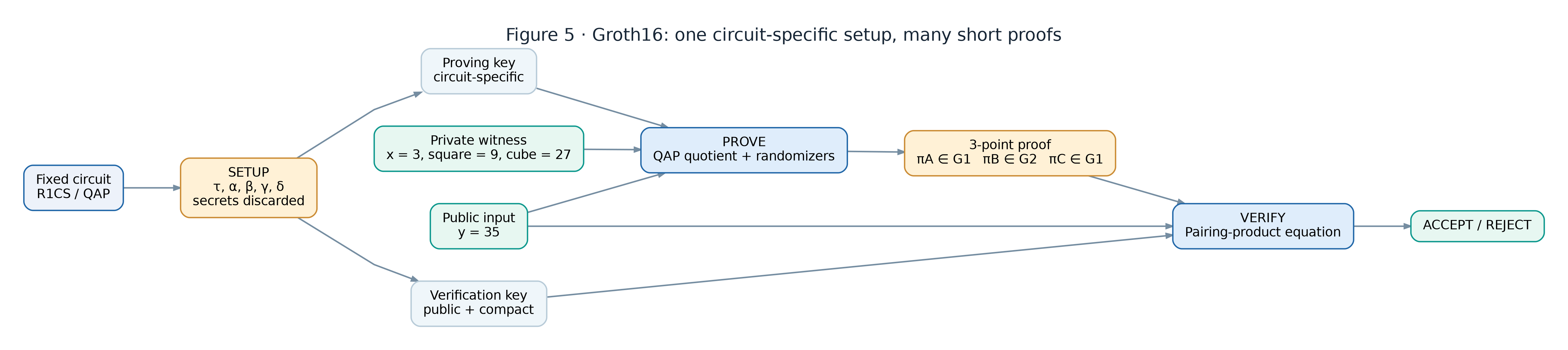
Groth16’s setup is specific to the circuit. It samples trapdoor scalars and emits a proving key and a verifying key. Anyone who keeps the trapdoor can forge, so a real ceremony destroys it. The lab leaves the trapdoors on screen so the cancellation is visible. The teaching values, in \mathbb{F}_{101}, are \tau = 7, \alpha = 13, \beta = 17, \gamma = 19, and \delta = 23.
A mnemonic, not a security theorem: \alpha and \beta tie the three proof components to one witness. \gamma scales the public terms the verifier computes. \delta scales the private-wire and quotient terms the prover computes. The split is what stops a prover from hiding a public claim inside the adjustable proof element. No single scalar does that job. The full key does.
The proof is three group elements:
The names collide with earlier letters. \pi_A, \pi_B, and \pi_C are not the R1CS matrices, and they are not the polynomials A_z, B_z, and C_z.
The verifier builds an accumulator from the verifying key and from the public inputs it intends to check, in order:
In this example the only public input is y, so the toy is V = \mathrm{IC}_0 + y\,\mathrm{IC}_1. The prover does not get to supply V in place of the verifier. V is not a fourth proof element.
The check is
Real verifiers often fold the right-hand side into one multi-pairing, sometimes with e([\alpha]_1, [\beta]_2) precomputed. The equation on its own does not list every proving-key encoding, and it does not establish knowledge soundness. Those come from the full construction and its assumptions.
The lab checks that same relation on the exponents, modulo 101. Fresh randomizers r and s enter the first two proof elements. Expanding the product adds cross terms. The formula for the third element carries the matching corrections, including an rs term, so the extra pieces cancel. Change r and s and the exponents move. A valid statement still verifies. That is completeness under randomization. It is the reason an honest randomized proof still passes. It is not, by itself, the zero-knowledge argument. Zero knowledge is a simulation claim about the whole protocol: the proof’s distribution can be produced without the witness.
Try it. The defaults are x = 3, r = 4, s = 8, and the verifier’s y = 35. Step to the check. It accepts. Press New randomizers and watch \pi_A, \pi_B, and \pi_C change while the result stays ACCEPT. Press Verify y + 1. The prover’s proof was built for 35. The verifier now uses 36, so V changes and this proof is rejected. Verify intended y accepts again. That rejection does not mean no proof exists for a different public output. It means this proof is bound to the statement the verifier asked about.
This module is not cryptography. It exposes the toy trapdoors and the scalar exponents. The field is small. There are no curve points and no pairings. A cheating prover who can see the exponents is not constrained the way Groth16 constrains one. The animation shows the cancellation that the group operations are there to check. It does not show that an untrusted setup is safe.
Changing the verifier’s y changes V even when the three proof elements stay put, because the verifier rebuilds V from its own input. New randomizers leave a valid statement verifiable because the third proof element carries the terms that cancel the new cross factors.
Where the zero knowledge sits
Zero knowledge protects the private witness relative to the public statement. It does not hide the statement. If y determines x, or if the field is small enough to search, the output has already leaked what you hoped to keep. Here the field has 101 elements. Hiding x from someone who is allowed to try all of them is not a security claim. It is a blackboard.
Succinct means the proof stays three group elements and the verifier’s pairing work stays constant as the circuit grows. Proving is the expensive direction. The verifier still reads every public input. It does one pairing product, not a pairing per gate and not a pairing per public input.
The narration sometimes splits the pairing equality into ordinary-language parts so a listener can hold it. Those parts are not separate tests. A proof generated for one statement normally fails if the verifier changes the public inputs. A new proof may exist for a different valid statement and a different witness. The public-input order and the verifying key have to be the ones the statement means.
What a developer should expect
A circuit-specific trusted setup is part of the system, not a deployment detail you can skip. The trapdoor randomness is either destroyed or kept under a ceremony whose assumptions you are willing to state. Shipping a new circuit means a new setup for that circuit.
The verifier checks the circuit you compiled. Missing constraints, missing range checks, and the wrong wire marked public all change the relation. Subgroup checks, the order of public inputs, and building V inside the verifier are part of an implementation. The scalar shadow does none of the cryptographic half of that list.
Groth16, as a pairing construction, falls if discrete log and pairings fall. That is the same limit called out for KZG openings in the Verkle essay. A hash-only argument does not have that particular dependency. This page does not compare proof systems beyond that. The worked example is the point.
Easy misreadings
| Layer | What it actually says | The tempting wrong reading |
|---|---|---|
| Field arithmetic | Circuit and QAP equations are modulo the scalar-field prime. | The numbers are ordinary unbounded integers. |
| Curve group | The group law is field arithmetic. The smooth drawing is one picture of it. | A finite-field curve is that drawing with the points snapped to pixels. |
| R1CS | Every row is checked against the same full assignment. | The witness is correct because some program computed it. |
| QAP | Vanishing at every designated point is the same claim as divisibility by Z. |
A check at one convenient point proves the program. |
| Reference string | Structured encodings let the prover make only certain combinations. | Publishing powers of τ is the whole security argument. |
| Randomizers | They change the proof and still verify for the same relation. | Cancellation by itself is the zero-knowledge proof. |
| Public input | The verifier builds V from the ordered statement it intends. |
The prover may send whatever accumulator it likes. |
| Soundness | It depends on the full setup and the stated assumptions. | Any numerical pairing equality is knowledge-sound. |
| Zero knowledge | The witness stays hidden beyond what the public statement already says. | A public output can never leak information. |
What to try next
Run the happy path once, in order. Add two field points. Run x = 3, y = 35 through the circuit. Confirm the R1CS residuals are [0, 0, 0]. Confirm the QAP remainder is zero. Accept the toy pairing check at y = 35.
Then break one layer at a time. In the circuit, change only public y. In R1CS, corrupt an internal wire. In the QAP, watch a nonzero residual become a nonzero remainder. In the Groth16 panel, keep the proof and change the verifier’s public input.
Then say the chain without the screen. A computation becomes wire constraints. A proposed witness has to satisfy every constraint. Interpolation puts each constraint at its own test point. All of them hold if and only if the error is divisible by the vanishing polynomial. Groth16 encodes that relation in curve-group elements, randomizes the proof, and lets the verifier check the pairing equation while binding the public inputs itself.
The Merkle and Verkle essay is the companion piece in the other direction: a root, a path, and an opening, with the pairing left as a pointer. This page was that pointer.
Sources
The episode’s arithmetic was checked against these. The lab’s field arithmetic and polynomial division run in the browser from the witness you type. They are not a playback of a fixed transcript.
- Jens Groth, On the Size of Pairing-Based Non-interactive Arguments (EUROCRYPT 2016).
- Alin Tomescu, Quadratic Arithmetic Programs and Rank-1 Constraint Systems, and Groth16.
- Zcash Halo 2 book, elliptic curves, and the Zcash notes on interactive proofs, zero knowledge, and SNARKs.
- bellman Groth16 verifier, including the pairing rearrangement.
- Penumbra, Groth16 recap, for the randomizers.
- Zcash protocol specification, Groth16 verification.